
이번 주는 머신러닝에 대해 배웠다...
수업시간에 한 것 복습도 좋지만... 프로젝트 때 해본 데이터에 적용을 해보려 한다!
데이터는 미니프로젝트때 만든 RFM데이터...
다!
우선 데이터 불러오면...
import pandas as pdrfm = pd.read_csv('data/rfm_classification.csv')
rfm
Recency(고객이 최근 구매한 날짜)
Frequency(고객이 물건을 산 날짜의 빈도)
MoneytaryValue(고객이 총 쓴 돈)
RFM_class(가중치를 적용해 갓 조은? 님이 만드신 유저별 등급)
Cluster(Kmeans알고리즘을 통해 만들어본 유저별 군집)
컬럼들이 있는데...
R, F, M, RFM_class로 Cluster를 분류하는 모델을 만들고자 한다!
사실 RFM_class도 RFM을 이용해 만든거고... Cluster도 RFM으로 만든거여서...
이게 사실 엉망스러운 분류를 한다! 지만...
나는... 초보 아기고양이...니까 데이터셋을 가지고 연습을 한다 치고 해보자!
일단 Cluster가 사실 카테고리인데 int타입이라 category형으로 바꿔주자!
rfm['Cluster'] = rfm['Cluster'].astype('category')
rfm.info()
음... R, F, M은 수치형이고 RFM_class는 범주형이니까...
걍 쉽게쉽게 스케일링은 생략하고... R, F, M은 머신러닝 그대로 돌리고 RFM_class는 인코딩 해주고 돌릴 거다!
일단 정답 데이터 컬럼명 적고...
label_name = 'Cluster'
label_name
y값 생성...
y = rfm[label_name]
y
그 다음...
X_raw(인코등 들어가기 전 문제데이터) 생성해주자!

shape확인도 함 해주고...
X_raw.shape, y.shape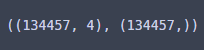
이제 train데이터와 test데이터를 나눠주면...
from sklearn.model_selection import train_test_split

X_train, X_test, y_train, y_test = train_test_split(X_raw, y, test_size=0.2, stratify=y, random_state=729)
8:2국룰로 나눠주고...
stratify=y로 정답이 균등하게 나눠지게끔 하고....
이런식으로... 해보면
X_train.shape, X_test.shape, y_train.shape, y_test.shape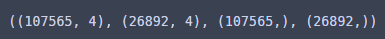
잘 나뉘었고...
정답의 분포도...
X_train.shape, X_test.shape, y_train.shape, y_test.shape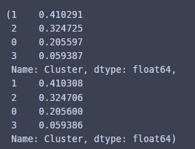
비슷비슷하다...
이제 범주형 데이터에 인코딩을 해볼건데...
rfm['RFM_class'].describe()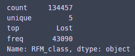
이렇게 클래스의 유일값이 5개니깐...
원 핫 인코딩 적용해 보자!
원 핫 인코딩할 컬럼 이름 불러와주고...
col_ohe = X_raw.select_dtypes(include='object').columns
col_ohe
원핫 인코딩 적용하고...
핸들언노운 이그노어 해 주면서...
test데이터는 fit 안 해 주면서...
shape까지 확인해보면...
from sklearn.preprocessing import OneHotEncoder

ohe = OneHotEncoder(handle_unknown='ignore')

X_train_ohe = ohe.fit_transform(X_train[col_ohe])
X_test_ohe = ohe.transform(X_test[col_ohe])
X_train_ohe.shape, X_test_ohe.shape
이렇게 클래스가 5개라 컬럼 5개로 잘 나뉘었다!
이제 원핫 인코딩한 것을 데이터프레임으로 바꿔주는데...
컬럼명 넣어 주면서...
인덱스 값도 까먹지 않고 넣어주면서...
train, test데이터 모두에 적용하면...
df_train_ohe = pd.DataFrame(X_train_ohe.toarray(), columns = ohe.get_feature_names_out())
df_train_ohe.index = X_train.index

df_test_ohe = pd.DataFrame(X_test_ohe.toarray(), columns = ohe.get_feature_names_out())
df_test_ohe.index = X_test.index

display(df_train_ohe)
display(df_test_ohe)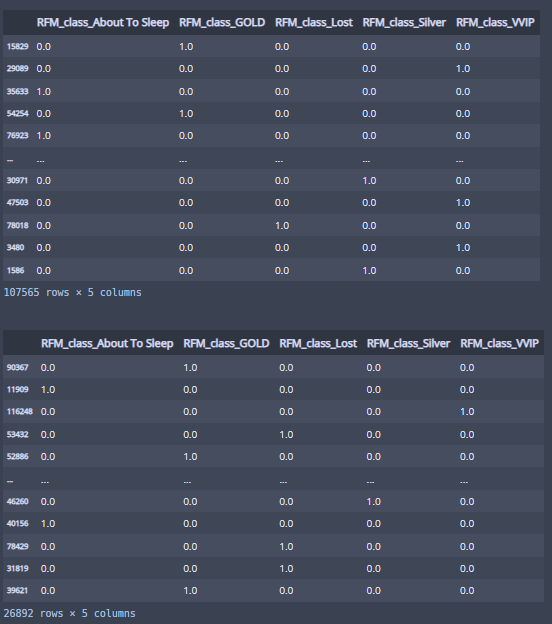
인코딩 완료! 해 주면서...
이제 수치형 데이터와 인코딩한 데이터를 합쳐서...
X_train_enc, y_train_enc에 넣어주면...
X_train_num = X_train.select_dtypes(exclude='object')
X_train_enc = pd.concat([X_train_num, df_train_ohe], axis=1)

X_test_num = X_test.select_dtypes(exclude='object')
X_test_enc = pd.concat([X_test_num, df_test_ohe], axis=1)

display(X_train_enc.head())
display(X_test_enc.head())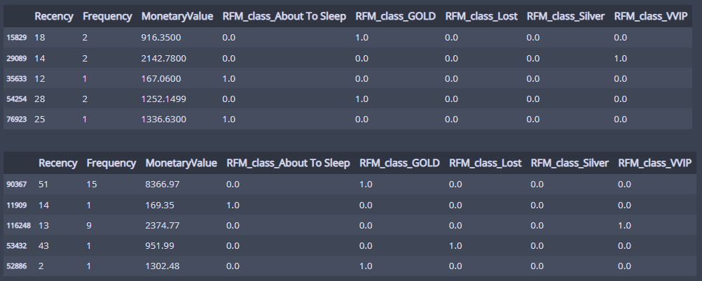
머신 러닝 들어가기 직전!...
이름부터 웅장
GradientBoostingClassifier만 써볼건데...
어차피 그리드 서치 해줄꺼니까...
대충 파라미터 넣고 만들어 버리면...
from sklearn.ensemble import GradientBoostingClassifier
model_gbc = GradientBoostingClassifier(learning_rate=0.2, n_estimators=100, random_state=729)
model_gbc
모델 생성!
그리드 서치에 파라미터 많이 넣어버리면... 컴퓨터가 아파해서...
걍 파라미터 각각 두개씩만 넣자...ㅜ
parameters = {'n_estimators':(100, 200),
              'learning_rate':(0.1, 0.2)}
parameters
그럼 GridSearchCV 돌려버리기!
cv=3(교차검증 분할 3개로 하고)
scoring은 분류모델이니까 accuracy로 해줬다!
from sklearn.model_selection import GridSearchCV
cla = GridSearchCV(model_gbc, parameters, cv=3, n_jobs=-1, verbose=2, scoring='accuracy')
cla.fit(X_train_enc, y_train)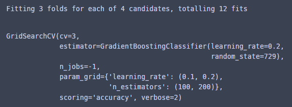
이거 웰케 오래걸리냐... 이거 맞냐...?
교차검증 분할 3개... 파라미터 2개에 각각 2개씩 넣어서 12번 돌아간 걸 알 수 있다...
암튼... best_model을 찾아보면...
best_model = cla.best_estimator_
best_model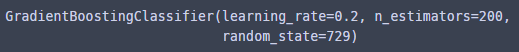
learning_late=0.2, n_estimators=200인 모델이 베스트 모델이구나...
그럼 모델 4에 대해 얼마나 좋은 모델인지 데이터프레임으로 보면...
pd.DataFrame(cla.cv_results_)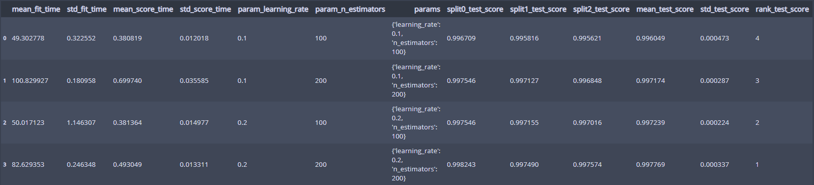
각 모델의 세부 정보를 볼 수 있다!
그럼 모델이 얼마나 정확한지 train데이터로 확인하기 위해서...
cross_val_predict로 best_model로 교차검증 해보자!
from sklearn.model_selection import cross_val_predict

y_valid_predict = cross_val_predict(best_model, X_train_enc, y_train, cv=3, n_jobs=-1, verbose=2)
y_valid_predict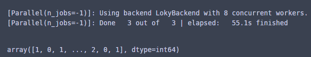
이렇게 y_valid_predict 검증할 정답값이 나왔고...
accuracy_score로 평가해보면...
from sklearn.metrics import accuracy_score
accuracy_score(y_train, y_valid_predict)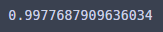
99,7퍼 넘게 맞췄다!
그럼 실제 테스트 셋으로 채점해보자!
best_model로 테스트 데이터로 예측해보면...
y_predict = best_model.predict(X_test_enc)
y_predict
채점할 답지 생성!
마지막 채점!
accuracy_score(y_test, y_predict)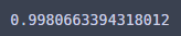
99.8이 조금 넘는다!
우리의 best모델의 feature_importance를 한번 보면...
fi = pd.Series(best_model.feature_importances_)
fi.index = best_model.feature_names_in_
fi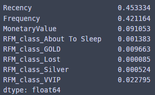
Recency가 가장 높다...? 흠...
그리고 About To Sleep, Lost, Silver 변수는 거의 영향을 안 준 것을 확인 할 수 있었고...
시각화도 해보면...
fi.plot.barh()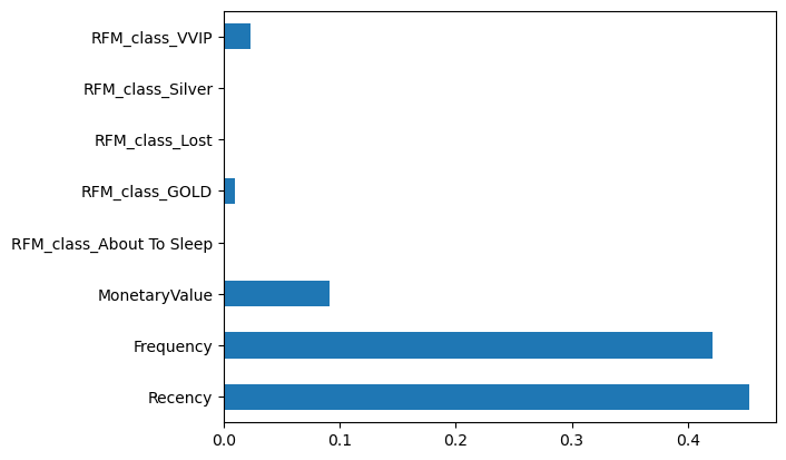
이 3개가 거의 안보여서...
좀 길게 보면...
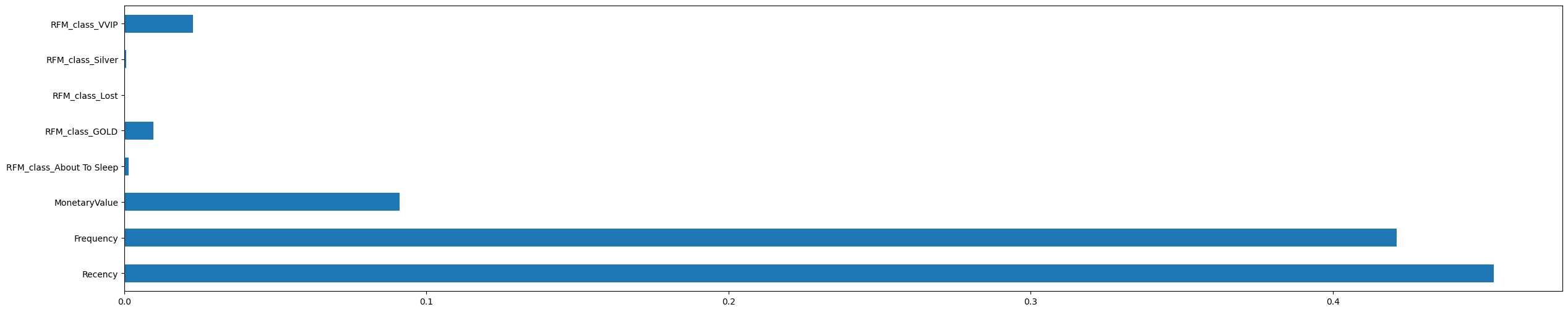
눈 크게 뜨고 봐야 보인다!
이번주에 배운 것을 사용해 가면서 해봤는데...
분류모델 그리드 서치가 생각보다 오래 걸려서 당황했지만...
그래도 한 번 해봤다는 거에 의미를....

'멋쟁이사자처럼 AI스쿨' 카테고리의 다른 글
| 멋쟁이사자처럼miniproject3(이커머스 데이터) (0) | 2023.03.19 |
|---|---|
| 멋쟁이사자처럼 AI스쿨 12주차 회고 (0) | 2023.03.09 |
| 과제3 심화? (0) | 2023.03.05 |
| 멋쟁이사자처럼 AI스쿨 11주차 회고 (0) | 2023.03.02 |
| 통계 특강5 (0) | 2023.03.02 |


댓글